An introduction to Boolean casting and vectorization in NumPy

Introduction

NumPy or “Numerical Python” is a powerful Python library that has risen to prominence for its extensive use cases in the scientific and data analysis communities. It is a free and open-source Python library that allows users to manipulate data through a simple-to-use and intuitive interface while simultaneously compensating for Python’s typical speed shortcomings via compiled C code on the back end.

Much like collecting as much logic as possible into a single list comprehension, the ability to avoid for loops in Python and instead do everything in NumPy (vectorization), has become a valuable skill in its own right.

This article will cover the basics of the NumPy array, which is the foundation on which all NumPy operations take place, as well as demonstrating boolean casting and how you can combine these into vectorizations for easy computation. But in order to demonstrate data manipulation we need some data to manipulate! In this case I have dug up a topic from my distant past: identifying stars from telescope images by their brightness. 15 years ago or so, when I did this at university, we had to do it by hand, and it took me a week and some horrible MATLAB to do properly. Now I’m a thirty-something programmer it should be a breeze! Right?

Step 0: the NumPy array

The “killer-app” object that the NumPy library introduces is the n-dimensional array (ndarray). It is an ordered, mutable, collection of values of a single type, that has to be an “orthotope” in shape (like a rectangle but with an arbitrary number of dimensions).

NumPy arrays are either created from existing collections or via various methods provided by the library, including things like arange, which produces a range of values, much like range in base Python.

In [33]: np.array([2,3,4])
Out[33]: array([2, 3, 4])

In [34]: np.arange(10)
Out[34]: array([0, 1, 2, 3, 4, 5, 6, 7, 8, 9])

Indexing in NumPy arrays is done via square parentheses similar to their distant list cousins. However, because these arrays are orthotopic, a simplified syntax is available for multiple dimensions. array[row_index, column_index, third_index, etc., ...].

In [13]: c = np.array([[0, 1, 2],
                       [3, 4, 5],
                       [6, 7, 8]])

In [15]: c[0, 0]
Out[15]: 0

In [16]: c[2, 1]
Out[16]: 7

It is also possible to get slices using this syntax and the list-slicing syntax :, like you would with lists.

In [17]: c[:, 0]
Out[17]: array([0, 3, 6])

In [18]: c[0, :]
Out[18]: array([0, 1, 2])

In [19]: c[1:-1,1:-1]
Out[19]: array([[4]])

Step 1: element-wise array operations

NumPy arrays have an extremely useful property. Compatible operations are evaluated element-wise between arrays. Which is to say, if you were to multiply two 1 x 3 arrays together, the result would be a 1 x 3 array with each element being the product of the two corresponding elements.

In [2]: import numpy as np

In [3]: a = np.array([1,2,3])

In [4]: a*a
Out[4]: array([1, 4, 9])

Only arrays of the same shape can be manipulated like this. What are the compatible operations? Almost all scalar operators work. Vector operators that depend on specific shapes, like the cross or dot product, do not. However, crucially expressions also work.

If instead of an operation, you created an expression (like x < 3) then the result will be a 3 x 3 boolean array which will have values of True where the expression is true and False where it is false.

In [5]: a > 2
Out[5]: array([False, False,  True])

Step 2: boolean casting

In NumPy the boolean arrays we constructed in the previous section can be used in place of indices in any array of the same shape (this is known as “boolean casting”), and only values corresponding to the True values will be returned.

In [4]: import numpy as np

In [5]: a = np.array([1,2,3])

In [6]: a[a >= 2]
Out[6]: array([2, 3])

In [7]: b = np.array(['h', 'e', 'l'])

In [8]: b[a >= 2]
Out[8]: array(['e', 'l'], dtype='<U1')

You can even chain expressions together using ~ for not, & for and, and | for or, as well as the correct parenthesis placement.

In [12]: b[(a <= 1) | (a > 2)]
Out[12]: array(['h', 'l'], dtype='<U1')

Boolean casting can be combined with slicing to do some really wacky selections. For example, we can combine our a and c examples.

In [13]: c = np.array([[0, 1, 2],
                       [3, 4, 5],
                       [6, 7, 8]])

In [23]: a = np.array([1, 2, 3])

In [24]: c[a > 2, :]
Out[24]: array([[6, 7, 8]])

You can go higher and more complex than this but remember that the shapes have to match the data that is being sliced. Boolean casting even works for assignment.

In [35]: c[a > 2, :]
Out[35]: array([[6, 7, 8]])

In [36]: c[a > 2, :] = 10

In [37]: c
Out[37]:
array([[ 0,  1,  2],
       [ 3,  4,  5],
       [10, 10, 10]])

The final piece of theory to know is that you may wish to use boolean casting in place of slicing for some applications, which can be done. However, when boolean arrays are cast as the only indices, the result will always be a flat array.

In [41]: x, y = np.indices((3,3))  # create x and y coordinate arrays of the given shape

In [42]: x
Out[42]:
array([[0, 0, 0],
       [1, 1, 1],
       [2, 2, 2]])

In [43]: y
Out[43]:
array([[0, 1, 2],
       [0, 1, 2],
       [0, 1, 2]])

In [44]: (x < 2) & (y < 2)
Out[44]:
array([[ True,  True, False],
       [ True,  True, False],
       [False, False, False]])

In [45]: c[(x < 2) & (y < 2)]
Out[45]: array([0, 1, 3, 4])

If you know that array would be orthotopic if reshaped, then you can get it back into the shape you want with np.reshape.

In [46]: d = c[(x < 2) & (y < 2)]

In [47]: d.reshape((2,2))
Out[47]:
array([[0, 1],
       [3, 4]])

Step 3: example application

That’s it! That’s technically all you need to know to use boolean casting, and hence vectorization, however I may as well say you’re now ready to write a novel now that you’ve mastered spelling and grammar as send you off into the world without anything further. Instead we’ll consider a simple example.

Consider this star map picture. This is a subsection of a much larger photo taken by a telescope. Which pixels are part of stars in this image? We could find out by hand but this is a small subsection of the original, so a programmatic solution is needed.

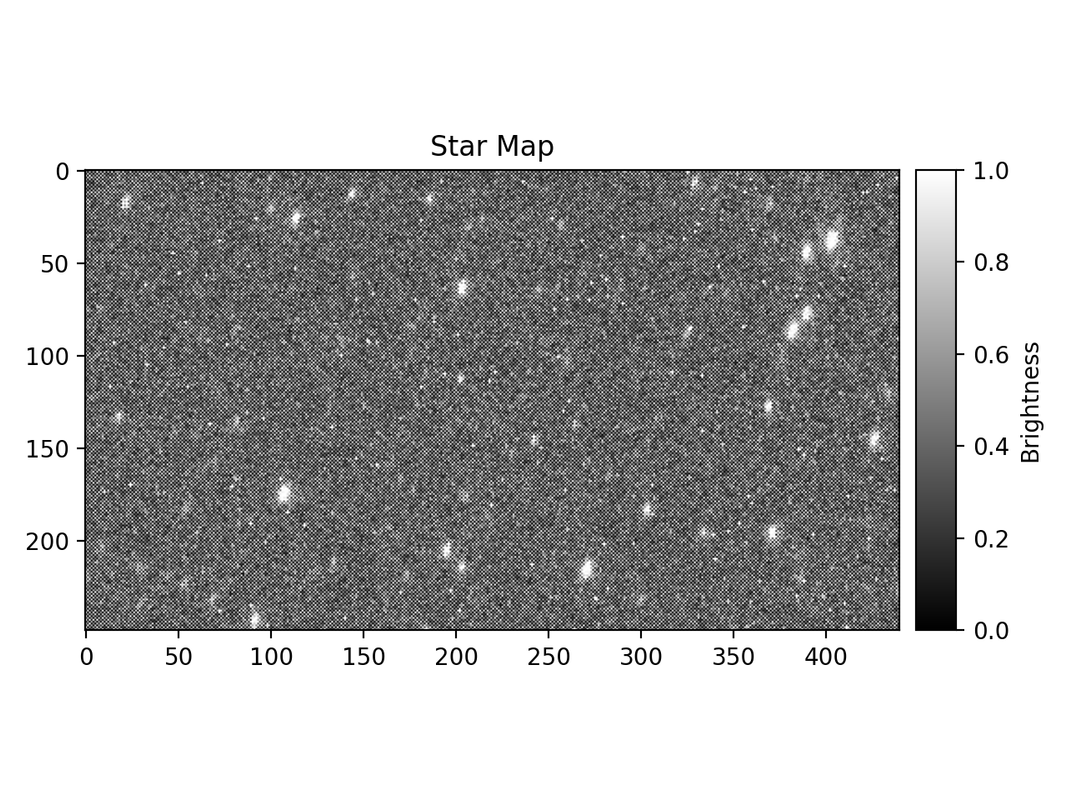
This star map is a subsection of Manual_60s60_Astro_20251003-234238661_27C.fits which was taken from https://nova.astrometry.net and made available under the Attribution 3.0 Unported license.

Thankfully, this telescope image is relatively simple data-wise as it is simply black and white. Each pixel is a measure of the brightness observed at that point (0 – 1). The process we’re going to follow to identify the stars is as follows.

• Load the image as a NumPy array
• Calculate the horizontal and vertical brightness gradients between each pixel
• Combine these using Pythagoras’ theorem to get the magnitude of the gradients
• Set all magnitudes above 0.1 to 1.0 to highlight regions of constant brightness
• Find the sum of all the neighboring pixel values to each pixel
• Pixel values with neighboring sums of less than 7 will be our stars!

In order to load the image as a NumPy array we need to make use of another member of the scientific python suite, matplotlib. This is the plotting library for scientific python and detailed use is beyond the scope of this article, but it’s a cool tool in its own right. All of the plotting in this article was done using Matplotlib and the main function is included at the bottom of the post. For now we will make use of the imread method.

First we need to load the telescope image as a NumPy array.

import matplotlib.pyplot as plt
import numpy as np



data = plt.imread('starmap.png')


print(type(data))
print(data.shape)
print(data)

Output:

<class 'numpy.ndarray'>
(249, 440)
[[0.03137255 0.4117647  0.06666667 ... 0.61960787 0.15686275 1.        ]
 [0.6431373  0.04313726 0.7176471  ... 0.28235295 0.6392157  0.        ]
 [0.02352941 0.8        0.02352941 ... 0.92156863 0.13333334 0.70980394]
 ...
 [0.07843138 0.8862745  0.07843138 ... 1.         0.         0.39215687]
 [1.         0.         0.63529414 ... 0.12156863 0.6666667  0.        ]
 [0.02745098 0.627451   0.         ... 0.93333334 0.         0.50980395]]

Neat!

The next step is to find the “brightness gradient” between pixels in the horizontal (x) and vertical (y) directions. The brightness gradient between pixels is simply the difference in value between adjacent pixels divided by the number of pixels of separation, which is just 1 in this case. To get a single number we take these gradients, square them and add them together like they are two sides of a triangle. This will also remove the need to worry about negative gradients as they will all necessarily be positive.

x_gradient_data = data[1:, :] - data[:-1, :]
y_gradient_data = data[:, 1:] - data[:, :-1]

magnitude_data = x_gradient_data[:, :-1]**2 + y_gradient_data[:-1,:]**2

It’s that simple! We calculate the gradients by taking the element-wise difference between two slices of the same data offset by one pixel and I have left out the unneeded division by one.

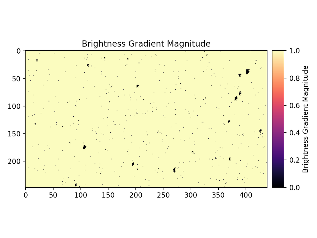
Next we only want to highlight flat gradients as the stars will be surrounded by relatively constant brightness, so let’s assign all gradients that are greater than 0.1 a value of 1.

magnitude_data[magnitude_data > 0.1] = 1

It’s beautiful how simple and concise it is. Although the next step is perhaps even better. We need the sum of every neighboring pixel’s gradient. Pixels surrounded by values of 1 will have a maximum value of 8, and those in our stars will have values of much less. In fact we can use this threshold to tune exactly how sensitive we want this algorithm to be. But how to calculate it?

To make the calculation we are going to employ the same principle as when we calculated the gradient, but using two for loops to ensure we iterate over all 8 possible neighbors (This is the only use of for loops in this article). We also use np.roll which shifts all values in the array in the direction specified by the amount specified (a single pixel here). In other words, at each iteration of the for loops the array is being “rolled” to that coordinate, providing just the right offset! An additional feature of roll that makes this whole thing possible is that cells at the edges of the array wrap around when it is used. Then the 8 arrays just have to be summed, and because it’s actually a generator this is all being done on demand, so the code isn’t producing 8 costly arrays at once either.

# Count number of neighboring 1s for each cell (8-neighborhood)
neighbors = sum(np.roll(np.roll(magnitude_data, i, 0), j, 1)
                for i in (-1, 0, 1)
                for j in (-1, 0, 1)
                if not (i == 0 and j == 0))

This is proper vectorization in action. Finally, we choose our threshold value to be 7 and get all the (x, y) coordinates where the neighbor count is less than 7 to be our stars.

neighbours[neighbors >= 7] = 8.


# np.where returns indices of the array supplied where the condition is True
# column_stack stitches the i, and j arrays that are returned into a single object.
star_coords = np.column_stack(np.where(neighbours < 8.))

# Simple scatter plot using Matplotlib with the star map underneath
fig, ax = plt.subplots()
ax.set_title('Detected Stars')
ax.imshow(data, cmap='binary_r', vmin=0., vmax=1.)
ax.scatter(x=star_coords[:, 1], y=star_coords[:, 0], c='red', s=1)
plt.show()

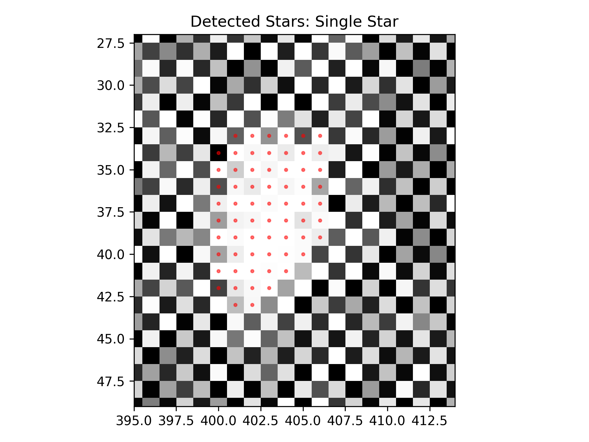
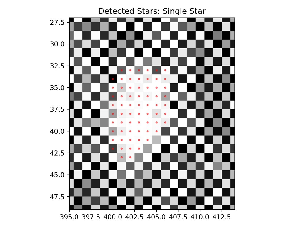
These results are a bit hard to see, so let’s look at the biggest star in the top-right of the image and see how we did. It is in a square of 395 < x < 414 and 27 < y < 49, and we can use boolean casting to get that section out.

yy, xx = np.indices(data.shape)
star_s1 = (395, 49)
star_s2 = (414, 27)
star_subsection = data[(
        (star_s1[0] < xx)
        & (xx <= star_s2[0])
        & (star_s1[1] > yy) #
        & (yy >= star_s2[1])
)]

… However, it would be a lot easier to just adjust the graph limits and replot and after doing so we can see the algorithm is identifying the pixels correctly!

Conclusion

In conclusion NumPy is an extraordinarily valuable Python library because it makes challenges like this possible to undertake in Python whilst also keeping the written code relatively readable and concise. Boolean casting in particular is at the core of what makes NumPy work best, as has been shown in this subsequent example. All the code used in this example can be found in this gist and the original star map photograph can be found at https://nova.astrometry.net.